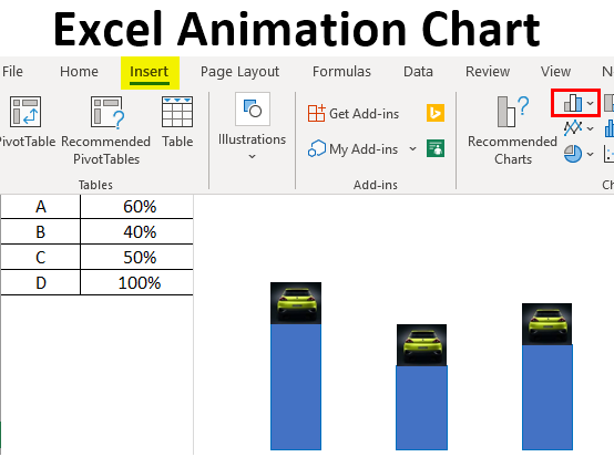
How To Create Animated Charts In Excel

Excel Animation Chart

Excel Animation Chart (Table of Contents)

Definition of Animation Chart in Excel
Example of Animation Chart in Excel

Introduction to Animation Chart in Excel

The charts that illustrate the data in an animated and dynamic way to better understand the charts are called animation charts. The animation charts require a little additional effort and knowledge of macro to create dynamic changes and movements in the chart.

To create an animation chart, we first need to create a normal chart for which we will add little coding to make it an animated chart. So, one should have knowledge of VBA coding to understand and create the animated charts. It is not mandatory to use coding for animated charts if you are good at creative thinking; you can also make it without VBA coding.

Example of Animation Chart in Excel

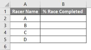
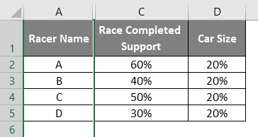
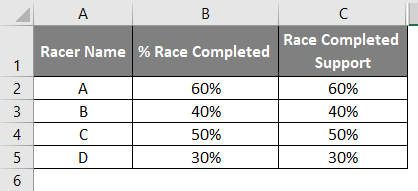
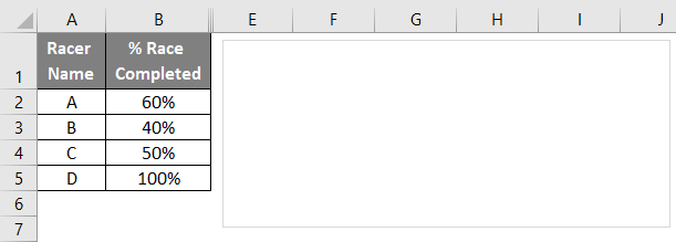
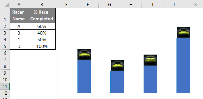
Here I am covering an example of percentage completion of race by a car. Follow the below steps to create the animated chart. First, create a small table layout for race details with racer name and percentage of Race completed as shown in the below picture.

You can download this Animation Chart Excel Template here – Animation Chart Excel Template

Excel Animation Chart 1-1

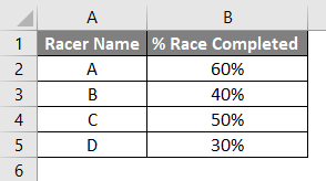
Enter the data related to the percentage of the race completed in "column B" if you want to input 60 percent input as 0.6 and then cntrl+shift+% symbol on the keyboard to convert to a percentage.

Excel Animation Chart 1-2

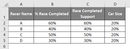
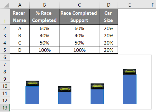
Now add another two columns as below and input the same data as column B. I know it may create confusion for you; it will clear once we create the chart.

Excel Animation Chart 1-3

Hide column B.

Excel Animation Chart 1-4

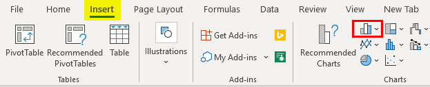
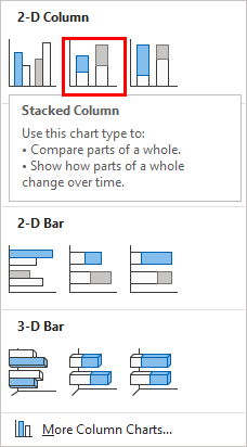
Select only visible data by clicking on Alt+; click on the Insert option, then choose 2D columns, which are highlighted in the red color box.

Excel Animation Chart 1-5

Select the Stacked Bar Chart below.

Excel Animation Chart 1-6

Excel Animation Chart 1-7

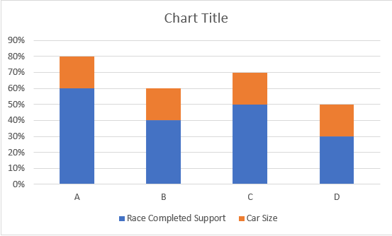
Now we will remove all the percentages, chart title and Legends by clicking on the plus symbol.

Excel Animation Chart 1-8

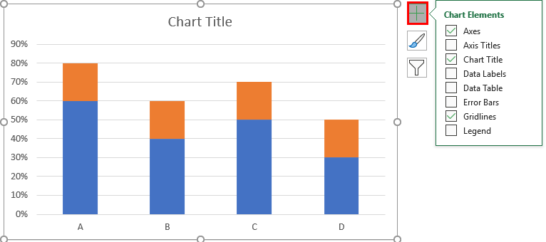
Deselect all the checkboxes below.

Excel Animation Chart 1-9

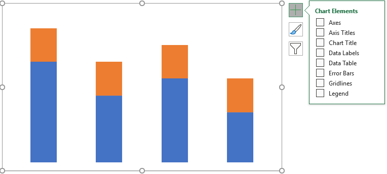
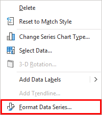
Click on right-hide on a chart, then select Format Data Series.

Format Data Series

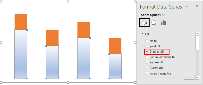
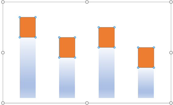
Now double click on the percentage completion part and choose Gradient fill on the right-hand side, as shown below. We can change the color as per our requirements.

Gradient Fill

Now choose the car percentage that is orange part of the chart as below.

Gradient Fill 1

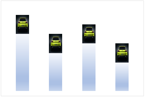
Choose a car picture from Google or copy a car picture that you have in your desktop images and paste it on the orange part; then, the map looks like below.

car picture

The design part of the chart is completed. Now, we need to complete the VBA coding to create movements to the cars when we ever change the percentage of completion of the race in the data table.

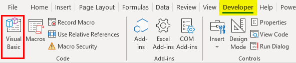
Click on the Developer tab and then click on the visual basic in the left-hand corner.

deveolper tab -Visual Basic

Click on the sheet in which you created the chart. Here my chart is in sheet 2.

visual basic code

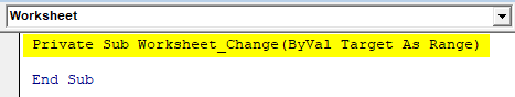
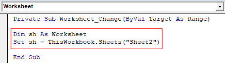
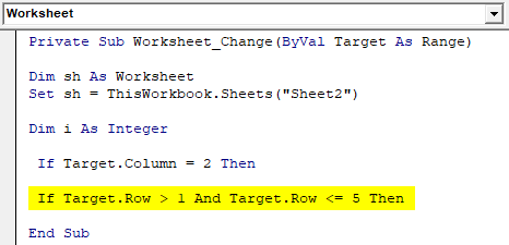
Select "Change" on the right top then we will get the "Private Sub Worksheet_Change(ByVal Target As Range)" in the coding area. The meaning of the code is, the program will run whenever we change the data. But we should write the program to run only when we change the particular set of data. For that, write the below coding.

Define a sheet "sh" and assign Sheet2 to sh as below.

Worksheet

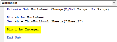
Define an integer as below.

Dim Integer

If we observe the data table, the "percentage race completed" column occupies column B and rows 2 to 5. So, our target is COLUMN B and ROWS 2 to 5.

Race Completed size

Once we clear about our target rows and columns, we will write the below coding. Check if the change is in column 2.

IF target

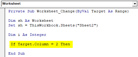
If it is column 2, then we need to check which row it is changing. The row should be 2 to 5, so write the below code.

IF target 1

If both the conditions satisfy, we need to perform an event as below.

Excel Animation Chart 1-8

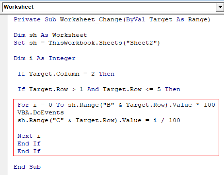
The meaning of the code is "i" value iterates from zero to a changed percentage value. That value will multiply by 100 because the value in the column is in percentage. After every value of "I", VBA will perform an event that is "I" value will divide by 100, and it will store in the same row but in column C, from where our chart is taking values with which appearance will change every time.

That means whenever we change the value in the percentage completion column, the value in column C starts from Zero and goes until the changed value(new value). After completion of the program, try to change the value in column B and observe the chart. You can observe the car movement from bottom to top depending on the percentage.

Racer name

Everything looks fine, but we have multiple columns of data is visible on the sheet. If you hide columns C and D, the chart also will disappear as below.

Racer name 1

The solution for this is to click, which will enable the "Design" menu on the top as below.

Selecting Data

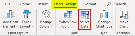
Select the option "Select Data", then a window will open as below.

Select Data Source

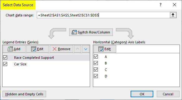
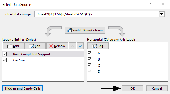
Click on the "Hidden and Empty cells" button.

Hidden and empty rows

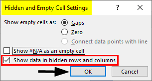
Check the option "Show data in hidden rows and columns", which will allow hiding the data related to charts. Select Ok here.

Race Completed support

Now hide the columns "C" and "D" and check.

% race completed

This is how we will make animated charts in excel. Similarly, we can make different kinds of animated charts like speedometer chart, circular charts, etc., in excel with the combination of our normal charts and VBA coding. All you need to do is creative ideas to design; there is no fixed way to create these animated charts.

Things to Remember

It is advisable to learn and understand the VBA coding to create a well-animated chart. But VBA coding is not that easy to write at the same to it does not require a computer science degree to learn.
Whenever creating an animated chart, try to keep it simple and clear because too much animation on unimportant data items also requires more coding or working may spoil the actual meaning.
Create the chart that apt for your data representation because every chart is not suitable for all situations. A wrong selection of chart may restrict you to represent a limited amount of data.
Don't forget to save excel with Macro enabled workbook when you use VBA coding.